Example 1: Runoff Calibration for the Dongjiang watershed

Background

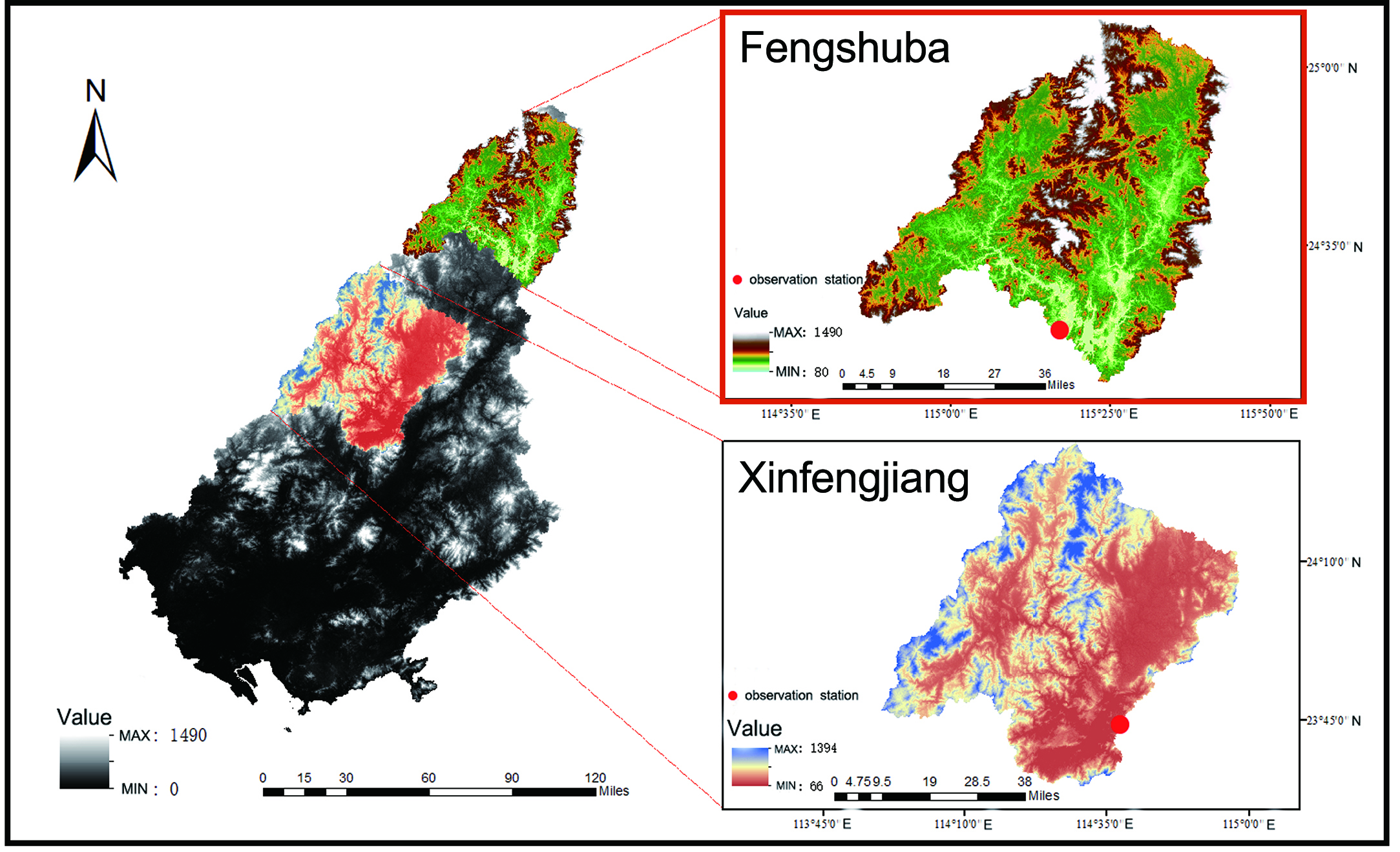
The Dongjiang watershed in Guangdong is a critical freshwater source, covering an area of over 35,000 square kilometers. It supplies water to several cities, including Guangzhou, Shenzhen, and Hong Kong.

In this study, we use the Fengshuba and XinFengJiang sub-basins of the Dongjiang watershed as examples for runoff calibration.

We primarily present the calibration process for the Fengshuba sub-basin, which has a catchment area of 5,150 km² and an average annual rainfall of 1,581 mm. But, for helping users familiar with SWAT-UQ, the calibration of the XinFengJiang sub-basin is provided as an additional exercise.

SWAT Modelling

For building SWAT model of Fengshuba sub-basin, the data set used includes:

DEM - The ASTER GDEM with a spatial resolution of 30 meters
Land Use - The RESDC (Resource and Environmental Science Data Center) dataset
Soil Data - The HWSD (Harmonized World Soil Database)
Meteorological Data - The CMADS (China Meteorological Assimilation Driving Dataset)
Observation - Runoff of Hydrographic Yearbook. (2008.1.1 to 2017.12.31)

For calibration, the simulation periods are:

Warm up Period - 2008.1.1 to 2011.12.31
Calibration Period - 2012.1.1 to 2016.12.31
Validation Period - 2017.1.1 to 2017.12.31

💡 Noted: Click this link to download project files.

Problem Define

The definition of the problem refers to the process of transforming a practical problem into an abstract problem that can be described using mathematical formulas and code.

In this example, the ultimate goal is to obtain the SWAT model whose output completely approximate to observed data. First, we need to identify the indicators to evaluate how well the SWAT model has been built. In hydrology, common indicators, e.g., NSE, R2, KGE, RMSE, PCC, and so on. Here, we use the NSE.

Therefore, this practical problem can be abstracted into:

Where $x$ denotes the undetermined parameters of the SWAT model; $NSE(\cdot)$ denotes the NSE operation; $sim$ denotes the simulation data obtained from running the SWAT model; $ob$ denotes the observed data from Chinese year book; $lb$ , $ub$ denotes the lower and upper bound of each parameters.

Next, based on this abstracted problem, we can describe it using code within the framework of SWAT-UQ.

Sensitivity Analysis

First, we would conduct sensitivity analysis (SA) for SWAT model. Refer to SWAT Manual and the article(Liu et al, 2017), following parameters are selected for SA.

ID	Abbreviation	Where	Assign Type	Range
P1	CN2	MGT	Relative	[-0.4, 0.2]
P2	GW_DELAY	GW	Value	[30, 450]
P3	ALPHA_BF	GW	Value	[0.0, 1.0]
P4	GWQMN	GW	Value	[0.0, 500.0]
P5	GW_REVAP	GW	Value	[0.02, 0.20]
P6	RCHRG_DP	GW	Value	[0.0, 1.0]
P7	SOL_AWC	SOL	Relative	[0.5, 1.5]
P8	SOL_K	SOL	Relative	[0.5, 15.0]
P9	SOL_ALB	SOL	Relative	[0.01, 5.00]
P10	CH_N2	RTE	Value	[-0.01, 0.30]
P11	CH_K2	RTE	Value	[-0.01, 500.0]
P12	ALPHA_BNK	RTE	Value	[0.05, 1.00]
P13	TLAPS	SUB	Value	[-10.0, 10.0]
P14	SLSUBSSN	HRU	Relative	[0.05, 25.0]
P15	HRU_SLP	HRU	Relative	[0.50, 1.50]
P16	OV_N	HRU	Relative	[0.10, 15.00]
P17	CANMX	HRU	Value	[0.0, 100.0]
P18	ESCO	HRU	Value	[0.01, 1.00]
P19	EPCO	HRU	Value	[0.01, 1.00]
P20	SFTMP	BSN	Value	[-5.0, 5.0]
P21	SMTMP	BSN	Value	[-5.0, 5.0]
P22	SMFMX	BSN	Value	[0.0, 20.0]
P23	SMFMN	BSN	Value	[0.0, 20.0]
P24	TIMP	BSN	Value	[0.01, 1.00]

As the tutorial introduce, we first prepare the parameter file:

File name: paras_sa.par

Name Mode Type Min_Max Scope
CN2 r f -0.4_0.2 all
GW_DELAY v f 30_450 all
ALPHA_BF v f 0.0_1.0 all
GWQMN v f 0.0_500.0 all
GW_REVAP v f 0.02_0.20 all
RCHRG_DP v f 0.0_1.0 all
SOL_AWC r f 0.5_1.5 all
SOL_K r f 0.5_15.0 all
SOL_ALB r f 0.01_5.00 all
CH_N2 v f -0.01_0.30 all
CH_K2 v f  -0.01_500.0 all
ALPHA_BNK v f 0.05_1.00 all
TLAPS v f -10.0_10.0 all
SLSUBSSN r f 0.05_25.0 all
HRU_SLP r f 0.50_1.50 all
OV_N r f 0.10_15.00 all
CANMX v f 0.0_100.0 all
ESCO v f 0.01_1.00 all
EPCO v f 0.01_1.00 all
SFTMP v f -5.0_5.0 all
SMTMP v f -5.0_5.0 all
SMFMX v f 0.0_20.0 all
SMFMN v f 0.0_20.0 all
TIMP v f 0.01_1.00 all

Then, the evaluation file should be created:

File name: obj_sa.evl

SER_1 : ID of series data
OBJ_1 : ID of objective function
WGT_1.0 : Weight of series combination
RCH_23 : ID of RCH, or SUB, or HRU
COL_2 : Extract Variable. The 'NUM' is differences with *.rch, *.sub, *.hru.
FUNC_1 : Func Type ( 1 - NSE, 2 - RMSE, 3 - PCC, 4 - Pbias, 5 - KGE, 6 - Mean, 7 - Sum, 8 - Max, 9 - Min )

1   2012 1 1    38.6
2   2012 1 2    16.2
3   2012 1 3    24.5
4   2012 1 4    26.9
5   2012 1 5    56.2
6   2012 1 6    82.1
7   2012 1 7    32.8
8   2012 1 8    20.5
9   2012 1 9    32.3
10  2012 1 10   28.9
11  2012 1 11   36.5
...
...
...
1821    2016 12 25  94.8
1822    2016 12 26  106
1823    2016 12 27  135
1824    2016 12 28  87.4
1825    2016 12 29  81.5
1826    2016 12 30  94.9
1827    2016 12 31  89.9

💡 Noted: Click this link to download related files(para_sa.par and obj_sa.evl)

Based on this evaluation file, SWAT-UQ would extract the data of Reach 23 from output.rch during 2012.1.1 to 2016.12.31. In addition, the NSE function is used to evaluate the performance of model outputs.

Finally, we can conduct the sensitivity analysis within python script-based environment:

from swat_uq import SWAT_UQ

projectPath = "E://swatProjectPath" # Use your SWAT project path
workPath = "E://workPath" # Use your work path
exeName = "swat2012.exe" # The exe name you want execute

#Blew two files should be created in the workPath
paraFileName = "paras_sa.par" # the parameter file you prepared
evalFileName = "obj_sa.evl" # the evaluation file you prepared

problem = SWAT_UQ(
   projectPath = projectPath, # set projectPath
   workPath = workPath, # set workPath
   swatExeName = exeName # set swatExeName
   paraFileName = paraFileName, # set paraFileName
   evalFileName = evalFileName, # set evalFileName
   verboseFlag = True, # enable verboseFlag to check if setup is configured properly.
   numParallel = 10 # set the parallel numbers of SWAT
)

# The SWAT-related Problem is completed. 

# Perform sensitivity analysis
from UQPyL.sensibility import FAST

fast = FAST()

# Generate sample set
X = fast.sample(problem = problem, N = 512)
# Therefore, the shape of X would be (12288, 24). It would be time-consuming to evaluate.

# Recommend: a. use Linux Serve Computer; b. use surrogate-based methods.

Y = problem.objFunc(X)

res = fast.analyze(X, Y)

print(res)

The analysis results of FAST methods are shown below:

We select the top 10 parameters to be calibrated, i.e., CN2, ALPHA_BNK, SOL_K, SLSUBBSN, ESCO, HRU_SLP, OV_N, TLAPS, SOL_ALB, CH_K2.

Optimization

Based on the above sensitivity analysis, we need to recreate parameter file:

File name: para_op.par

Name Mode Type Min_Max Scope
CN2 r f -0.4_0.2 all
SOL_K r f 0.5_15.0 all
SOL_ALB r f 0.01_5.00 all
CH_K2 v f  -0.01_500.0 all
ALPHA_BNK v f 0.05_1.00 all
TLAPS v f -10.0_10.0 all
SLSUBSSN r f 0.05_25.0 all
HRU_SLP r f 0.50_1.50 all
OV_N r f 0.10_15.00 all
ESCO v f 0.01_1.00 all

The evaluation file is the same as the SA. But it is a good habit to rename it to obj_op.evl

💡 Noted: Click this link to download related files(para_op.par, obj_op.evl and val_op.evl for validation).

Finally, we can run the optimization within python script-based environment:

from swat_uq import SWAT_UQ

projectPath = "E://swatProjectPath" # Use your SWAT project path
workPath = "E://workPath" # Use your work path
exeName = "swat2012.exe" # The exe name you want execute

#Blew two files should be created in the workPath
paraFileName = "paras_sa.par" # the parameter file you prepared
evalFileName = "obj_sa.evl" # the evaluation file you prepared

problem = SWAT_UQ(
   projectPath = projectPath, # set projectPath
   workPath = workPath, # set workPath
   swatExeName = exeName # set swatExeName
   paraFileName = paraFileName, # set paraFileName
   evalFileName = evalFileName, # set evalFileName
   verboseFlag = True, # enable verboseFlag to check if setup is configured properly.
   numParallel = 10 # set the parallel numbers of SWAT
)

# The SWAT-related Problem is completed. 

from UQPyL.optimization import PSO

pso = PSO(nPop = 50, maxFEs = 30000, verboseFlag = True, saveFlag = True)

pso.run(problem = problem)

The optimization results show:

We list the optimal decision with NSE->0.88:

CN2	SOL_K	SOL_ALB	CH_K2	ALPHA_BNK	TLAPS	SLSUBSSN	HRU_SLP	OV_N	ESCO
-0.236	14.278	0.325	46.604	1.000	-5.532	1.611	0.515	3.162	0.010

Validation

We have obtained the optimal parameter settings for the SWAT model. Now, we proceed to perform validation.

The evaluation file must first be prepared. Here, we apply the observed data ranging from 2017.1.1 to 2017.12.31.

File name: val_op.evl

SER_1 : ID of series data
OBJ_1 : ID of objective function
WGT_1.0 : Weight of series combination
RCH_23 : ID of RCH, or SUB, or HRU
COL_2 : Extract Variable. The 'NUM' is differences with *.rch, *.sub, *.hru.
FUNC_1 : Func Type ( 1 - NSE, 2 - RMSE, 3 - PCC, 4 - Pbias, 5 - KGE, 6 - Mean, 7 - Sum, 8 - Max, 9 - Min )

1 2017 1 1 74.4
2 2017 1 2 99.4
3 2017 1 3 77.4
...
...
365 2017 12 31 19.1

Using a Python script-based environment, we conduct the validation as follows:

# optima
X = np.array([-0.236, 14.278, 0.325, 46.604, 1.000, -5.532, 1.611, 0.515, 3.162, 0.010])

# Perform validation
# `problem.validate_parameters` expects the optimized parameters and the validation file.
# It returns a dictionary containing two keys: 'objs' (objective values) and 'cons' (constraint violations).
res = problem.validate_parameters(X, valFile = "val_op.evl") 

# Print the objective function values from the validation results
print(res["objs"])

Apply optima to project

Now, we need to apply these values to the project folder:

# Optimal parameter values
X = np.array([-0.236, 14.278, 0.325, 46.604, 1.000, -5.532, 1.611, 0.515, 3.162, 0.010])

# Apply parameters
problem.apply_parameters(X, replace=False)  
# Setting 'replace=False' will apply the values to the working directory without modifying the original project files.

# Alternatively
problem.apply_parameters(X, replace=True)  
# Setting 'replace=True' will overwrite the original project folder, which is not recommended.

So far, the calibration work is completed.

Exercise for users

We provide an exercise based on the Xinfengjiang sub-basin, which is part of the Dongjiang watershed.

You can download the complete project files here: Click here to download project files

Within the downloaded project files, the observed data is stored in the file named observed.txt.

If you have any questions or need assistance, feel free to contact us.